← All research and insights

From circuit tracing to input-token importance

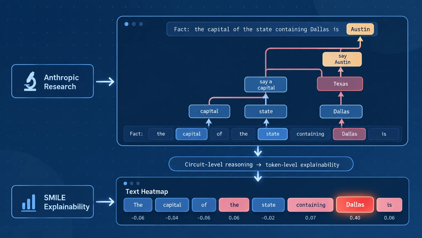
Select the image to open it at full resolution.

LLM interpretability · XWhy explainer · Circuit tracing, attribution graphs and token attribution

In short

Input-token importance is the projection of a circuit-tracing attribution graph onto the prompt. Start from the target output node, follow every weighted path backwards until it reaches an input embedding, add up the influence that arrives at each token, keep the unexplained error share separate, and normalise. The result is a token heatmap that is directly comparable with SMILE, SHAP, LIME or Integrated Gradients, but it inherits the mechanistic grounding of the graph.

Ask a language model to complete "Fact: the capital of the state containing Dallas is" and it answers Austin. Nowhere in the prompt does the word Texas appear. Somewhere inside the model, Dallas had to become Texas, and Texas combined with capital had to become Austin.

In 2025, Anthropic's interpretability team made that hidden hop visible. Their papers Circuit Tracing: Revealing Computational Graphs in Language Models and On the Biology of a Large Language Model introduced attribution graphs, which are maps of the interpretable features a model uses on one prompt and of how those features push on each other. The Dallas example became one of the best-known pictures in interpretability, retold in Anthropic's accessible essay Tracing the thoughts of a large language model. The tooling was later released as the open-source circuit-tracer library, with an interactive graph explorer on Neuronpedia (announcement).

Most people who use explainability in practice ask a simpler question, though: which words in my prompt mattered? This is input-token explainability, the question answered by tools such as XWhy's LLM explainer, SHAP, LIME and Integrated Gradients. This article explains how the two views connect. It shows how to read an attribution graph and turn it into a ranked list of input tokens in five steps. It also explains when you should prefer one view over the other.

Two questions, two kinds of answer

	Circuit tracing (attribution graph)	Input-token explainability
Question	How did the model compute the answer?	Which input tokens drove the answer?
Output	A graph of features, intermediate concepts and weighted edges	One score per prompt token
Access needed	White-box: weights, activations and trained transcoders	Black-box (SMILE, LIME, SHAP) or gradients (Integrated Gradients)
Strength	Reveals multi-step reasoning, such as Dallas → Texas → Austin	Compact, comparable and easy to evaluate and report
Weakness	Large, model-specific and time-consuming to read	Hides why a token matters and which route it took

Neither view replaces the other. A token heatmap can tell you that Dallas mattered, but not that it mattered because the model internally retrieved Texas. A graph shows the route, but with hundreds of nodes it is hard to compare across prompts, models or explainers. Collapsing the graph onto the input tokens provides a mechanistically grounded token score, and that score can be checked against perturbation-based explainers.

Step 1: Decide what you want from the graph

Step 1: read the intervention graph. Purple nodes are input embeddings, blue nodes are internal concepts and the green node is the target, Say Austin. The 2× / −2× labels are interventions, not importance. The goal is to measure how much each prompt token contributed to predicting Austin.

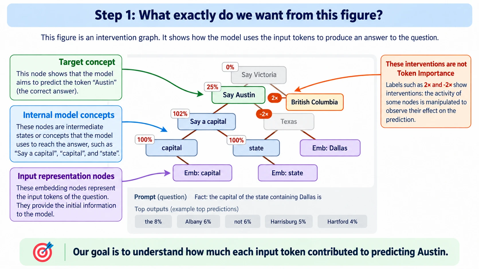
The figure is an intervention graph for the Dallas prompt. Read it from the bottom up:

• Input representation nodes (Emb: capital, Emb: state, Emb: Dallas) are the token embeddings. Every piece of information the model uses begins here.
• Internal model concepts, such as capital, state, Texas and Say a capital, are interpretable features found by the replacement model's transcoders.
• The target concept, Say Austin, is the feature cluster that pushes the logit for Austin.

The labels 2× and −2× and the percentages are interventions. In the original experiment, the researchers suppressed the Texas features and injected British Columbia features, and the model's answer moved from Austin to Victoria. These experiments show that the circuit is causal, but they are not token importance. Keep them aside for validation. The quantity you want is a number for each prompt token that says how much it contributed to Austin.

Step 2: Find where the inputs enter the graph

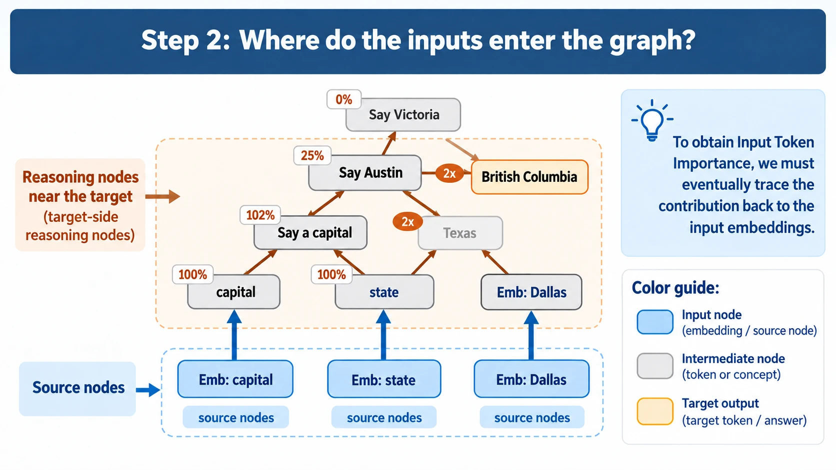
Step 2: find the source nodes. Every contribution to the answer enters the graph through an embedding node, so token importance must be traced all the way back to Emb: capital, Emb: state and Emb: Dallas, not just to the reasoning nodes near the target.

In an attribution graph, information flows from sources to the target. The source nodes are the embedding nodes, one for each prompt position. The reasoning nodes near the target sit in the middle. They are the most interesting part of the circuit, but they are not the inputs.

This matters for the conversion. The graph shows direct edges such as capital → Say a capital, but a token score must include all indirect influence that starts at a token's embedding and eventually arrives at the output. Looking at the top of the graph alone would miss that influence.

In the circuit-tracer implementation, the adjacency matrix stores nodes in a fixed order: [active features, error nodes, embedding nodes, logit nodes]. Rows are targets and columns are sources. The embedding block therefore contains one column for each input token, which gives you the token axis directly.

Step 3: Trace every path back from the target

Step 3: trace every path from the target back to the inputs. capital works through Say a capital, while state and Dallas both work through Texas. A token's importance is the sum over all of its paths, not any single edge.

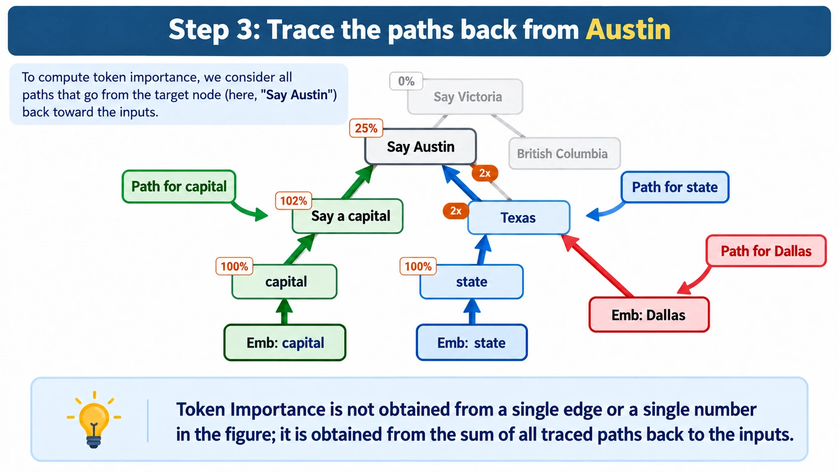
To score a token, consider every path from the target node (Say Austin) back to that token's embedding:

• capital: Emb: capital → capital → Say a capital → Say Austin
• state: Emb: state → state → Texas → Say Austin
• Dallas: Emb: Dallas → Texas → Say Austin

The influence along one path is the product of its normalised edge weights. The influence of a token is the sum over all of its paths. The token score is therefore not one edge or one number read from the figure. It is the combined result of every traced route.

In matrix form, let A be the adjacency matrix with each row normalised by the absolute values of its incoming weights. Paths of length k are captured by A^k, so the total influence over paths of every length is:

B = A + A² + A³ + … = (I − A)⁻¹ − I

This is the same indirect influence computation that Anthropic uses to prune attribution graphs. It appears as compute_influence in circuit-tracer's graph.py.

Step 4: Add up each input's contribution, and keep the error separate

Step 4: add up everything that reaches each embedding. Each token gets the sum of the contributions from all paths ending at it. The part the replacement model cannot explain is kept as a separate error share and is not assigned to any token.

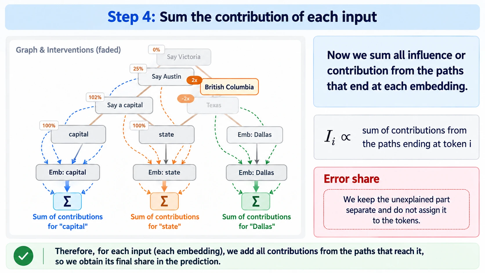
Weight the output logits by their probabilities, propagate that weight through B and read off the embedding columns. This gives the raw importance of each token:

I_i ∝ Σ_{paths Embi → target} Π_{edges on path} Ã_edge

The error share is where this method differs from most token heatmaps. Circuit tracing replaces the model's MLPs with transcoders, and the replacement is imperfect. The part it cannot reconstruct is represented by error nodes. Some of the output's influence flows through those error nodes, and that influence cannot be honestly assigned to any token. A faithful conversion therefore reports the error share as a separate bucket and does not spread it across the tokens. Gradient and perturbation methods have no equivalent of this explicit, measured uncertainty.

Step 5: Normalise to get input-token importance

Step 5: normalise to get input-token importance. capital (0.271), Dallas (0.181), containing (0.137) and state (0.118) carry most of the weight, and function words stay near zero. The bars sum to 0.812, and the remainder is the error share.

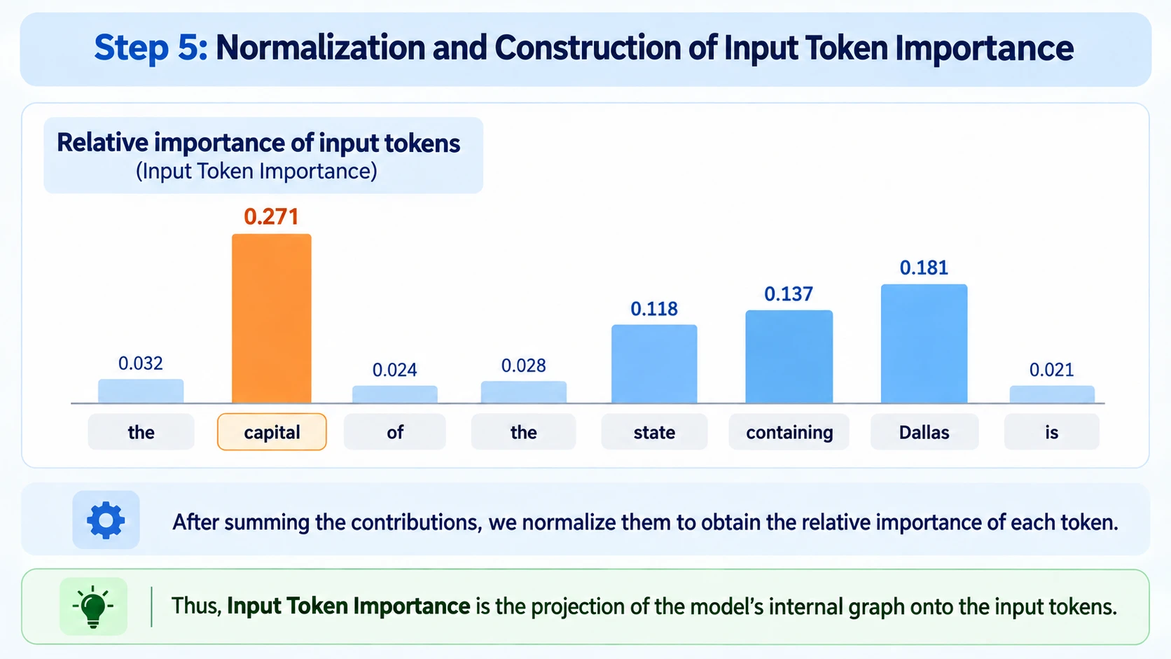
Finally, divide by the total influence that reaches the inputs, including the error nodes:

Î_i = I_i / (Σ_j I_j + I_error)error share = I_error / (Σ_j I_j + I_error)

In the illustrative example, the token scores add up to 0.812, so about 19% of the influence remains unexplained. That leftover is the error share, and you should report it alongside the heatmap. The ranking follows the circuit:

1. capital (0.271) selects the Say a capital pathway. Without it, the model has no reason to produce a city.
2. Dallas (0.181) is the only source of Texas, which the model has to work out for itself.
3. containing (0.137) and state (0.118) define the relation "the state that contains X".
4. Function words such as the, of and is receive little weight.

The ratio Σ_i I_i / (Σ_i I_i + I_error) is exactly what circuit-tracer calls the graph's replacement score. The token importance vector is therefore the per-token breakdown of a quality metric the library already computes.

Try it with circuit-tracer

Run it on Kaggle

You can try this code without installing anything. The Circuit Tracing → Token Importance notebook on Kaggle runs the code from this section, so you can see the token-importance results for yourself.

The sketch below uses the public circuit-tracer API with Gemma-2-2B and its released transcoders. Node ordering follows the library's Graph class.

import torch
from circuit_tracer import ReplacementModel, attribute
from circuit_tracer.graph import normalize_matrix, compute_influence

model = ReplacementModel.from_pretrained("google/gemma-2-2b", "gemma", dtype=torch.bfloat16)
prompt = "Fact: the capital of the state containing Dallas is"
graph = attribute(prompt=prompt, model=model, max_n_logits=10, desired_logit_prob=0.95)

n_tokens = len(graph.input_tokens)
n_logits = len(graph.logit_targets)
n_features = len(graph.selected_features)
error_start, error_end = n_features, n_features + n_tokens * graph.cfg.n_layers
token_end = error_end + n_tokens

# Weight each output logit by its probability, then propagate through all paths.
logit_weights = torch.zeros(graph.adjacency_matrix.shape[0])
logit_weights[-n_logits:] = graph.logit_probabilities
influence = compute_influence(normalize_matrix(graph.adjacency_matrix), logit_weights)

token_influence = influence[error_end:token_end]            # one value per input token
error_influence = influence[error_start:error_end].sum()    # kept separate
total = token_influence.sum() + error_influence

importance = (token_influence / total).tolist()
tokens = [model.tokenizer.decode(t) for t in graph.input_tokens]
for tok, score in zip(tokens, importance):
    print(f"{tok!r:>14}  {score:.3f}")
print(f"{'error share':>14}  {(error_influence / total).item():.3f}")

To attribute a single answer, such as Austin on its own instead of the top-k logit mix, pass that token through attribution_targets and keep only its logit weight. Before you rely on the numbers, open the Dallas → Austin graph on Neuronpedia and check the paths yourself.

How does this compare with other token-attribution methods?

Method	What it measures	Access	Handles multi-hop reasoning?	Reports what is unexplained?
Circuit-traced token importance	Path-summed influence through interpretable features	White-box + transcoders	Yes, explicitly (via Texas)	Yes (error share)
SMILE / gSMILE (XWhy)	Local surrogate fitted to output changes under prompt perturbations	Black-box, works with API models	Implicitly	Via surrogate fit (R², fidelity)
LIME / SHAP	Local surrogate or Shapley value of token presence	Black-box	Implicitly	Partially (fit / additivity)
Integrated Gradients	Path integral of gradients from a baseline	Gradients	No	Completeness axiom only
Attention rollout	Propagated attention weights	Attention maps	No, and attention is not the whole computation	No

The main distinction is that perturbation methods such as SMILE observe what happens when a token is removed, whereas circuit tracing reads how the model computes with it. When both methods rank capital and Dallas first, you have two independent lines of evidence. When they disagree, you have found something worth investigating. Possible causes include a high error share, redundant pathways that hide a token's effect when it is removed, or a perturbation scheme that creates unnatural prompts. For concrete checks, see Does the explanation hold up? and XWhy's ATT faithfulness metric.

Limits worth stating

• The heatmap describes the replacement model, not the original model. Attribution graphs are computed on a transcoder-based replacement model with frozen attention patterns. The error share tells you how far that replacement is from the original.
• Magnitude is not sign. Normalising absolute edge weights mixes excitatory and inhibitory influence. If you need to know whether a token pushed towards or pushed away from the answer, keep signed paths separately.
• Collapsing the graph loses the route. A heatmap shows that Dallas mattered but not that it worked through Texas. Publish the graph link together with the token scores.
• The explanation is local. Like any local explanation, this one describes one prompt, one model and one set of transcoders.
• Interventions are validation, not attribution. Use the 2× / −2× steering experiments to test the explanation, as Anthropic did with Texas → British Columbia → Victoria, rather than as importance scores.

Frequently asked questions

What is circuit tracing? Circuit tracing is a mechanistic interpretability method from Anthropic. It replaces a language model's MLP layers with interpretable transcoder features and builds an attribution graph that shows how those features, the input tokens and the output logits influence one another on a single prompt. The method is described in Circuit Tracing and implemented in circuit-tracer.

Can circuit tracing produce input-token importance? Yes. Sum the indirect influence from the target output to each input-embedding node over all paths, keep the error-node influence separate and normalise. The per-token scores sum to the graph's replacement score, and the remainder is the error share.

How is this different from SHAP, LIME or SMILE? SHAP, LIME and SMILE are black-box methods that perturb the prompt and fit a local surrogate to the observed changes in the output. Circuit-traced token importance is white-box: it follows the model's internal computation. The two are complementary, and agreement between them is strong evidence that an explanation is faithful.

Why keep the error share separate instead of spreading it across tokens? The error nodes represent computation that the replacement model does not explain. Assigning that influence to tokens would overstate how much you know. Reporting it separately makes the uncertainty explicit.

Which models can I trace? circuit-tracer supports open-weight models that have released transcoders, including Gemma-2 (2B), Gemma-3, Llama-3.2 (1B) and Qwen3 (0.6B–14B). You can explore pre-computed graphs on Neuronpedia. For closed API models, use a black-box explainer such as XWhy's LLM explainer.

Further reading

• Anthropic, Circuit Tracing: Revealing Computational Graphs in Language Models (2025), the method paper.
• Anthropic, On the Biology of a Large Language Model (2025), the source of the Dallas → Austin case study.
• Anthropic, Tracing the thoughts of a large language model, an accessible overview.
• Anthropic, Open-sourcing circuit tracing tools, and the safety-research/circuit-tracer repository.
• Anthropic, Mapping the mind of a large language model and Scaling Monosemanticity, the background on interpretable features.
• Dunefsky, Chlenski and Nanda, Transcoders find interpretable LLM feature circuits (2024).
• Kaggle notebook: Circuit tracing → token importance, a runnable version of the code in this article with its outputs.
• On the XWhy site: Explaining LLM responses, How SMILE works, the LLM explainer guide and the gSMILE preprint.